TEECNet and MegaFlow2D

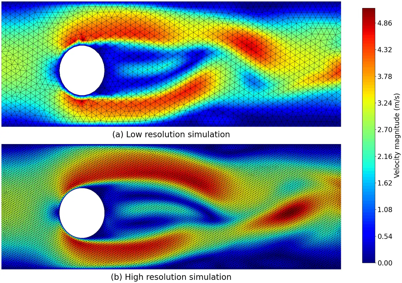
Carnegie Mellon University · Design Research Collective · 2022 – 2025 · presented at APS-DFD 2023, Washington DC

A cylinder wake velocity field shown twice: above on a coarse triangular mesh where the wake is smeared, below on a fine mesh where the shear layers are sharp. Mesh edges are visible in both.

Both panels above are the same flow past the same cylinder. The top one ran quickly on a coarse mesh and smeared the wake into the free stream; the bottom one resolved it and cost far more. Refining a mesh buys accuracy at a price that climbs steeply, and that trade is the reason high-fidelity CFD sits outside most design loops.

30train/test resolution pairs, one architecture 0.95–0.9995R² when trained on [20,40] or finer 3.2×faster than the neural-operator baseline on 12 cores

Learn the error, not the answer

The gap between a coarse and a fine solution is discretization error, and unlike most things a network is asked to predict, theory already says something about it: a power series in the cell size, with an order of accuracy set by the scheme. TEECNet takes that expression and replaces its unknown coefficient with a learned approximator, instead of learning the coarse-to-fine map from scratch.

That change of target is the whole design. The solution field is large, sharp and globally coupled; the error field is smaller, smoother and mostly local. TEECNet asks the network for the easier of the two objects, on a target whose behaviour theory already constrains.

And the coefficient has to be learned rather than derived. Observed order of accuracy tracks theory well for global quantities — integrate over a whole surface and it behaves — but correlates inconsistently with theory for local ones. That inconsistency is precisely the gap a learned coefficient fills.

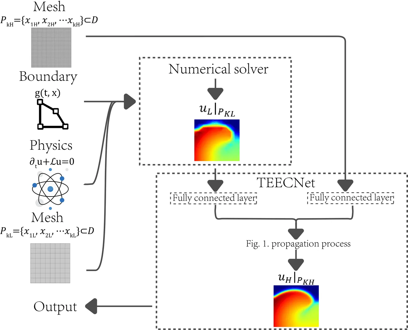
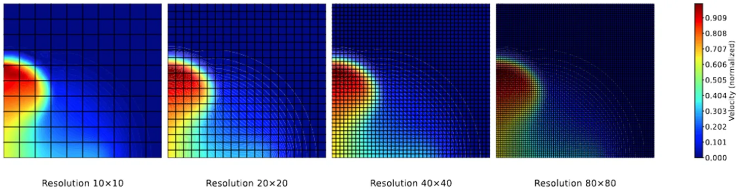
Pipeline diagram: a low-resolution mesh, boundary conditions and the governing physics feed a numerical solver; its coarse solution and the high-resolution mesh both feed TEECNet, which outputs the high-resolution field. — The coarse solution and the fine mesh both enter TEECNet; error is estimated on every mesh edge from its neighbouring nodes, then aggregated back onto each node. Nothing in that loop assumes a grid.

It is not that the model tolerates unstructured meshes; it never knew what kind of mesh it was on.

What actually happened

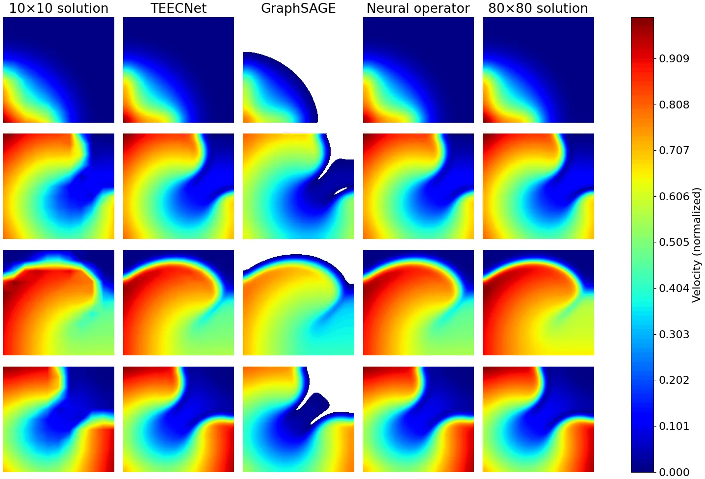
The same advection-diffusion solution drawn on four grids of increasing density, 10 by 10 through 80 by 80, with the plume front sharpening from left to right. — The same advection–diffusion solution on 10×10 through 80×80. Watch the plume front go from blocky to sharp — that is the gap the correction has to close.

Against a general-purpose graph network the difference is not subtle. GraphSAGE tears holes in the domain — white voids, missing wedges — because nothing obliges it to respect the physics it is interpolating through. TEECNet matches the neural operator’s accuracy and beats it on cost.

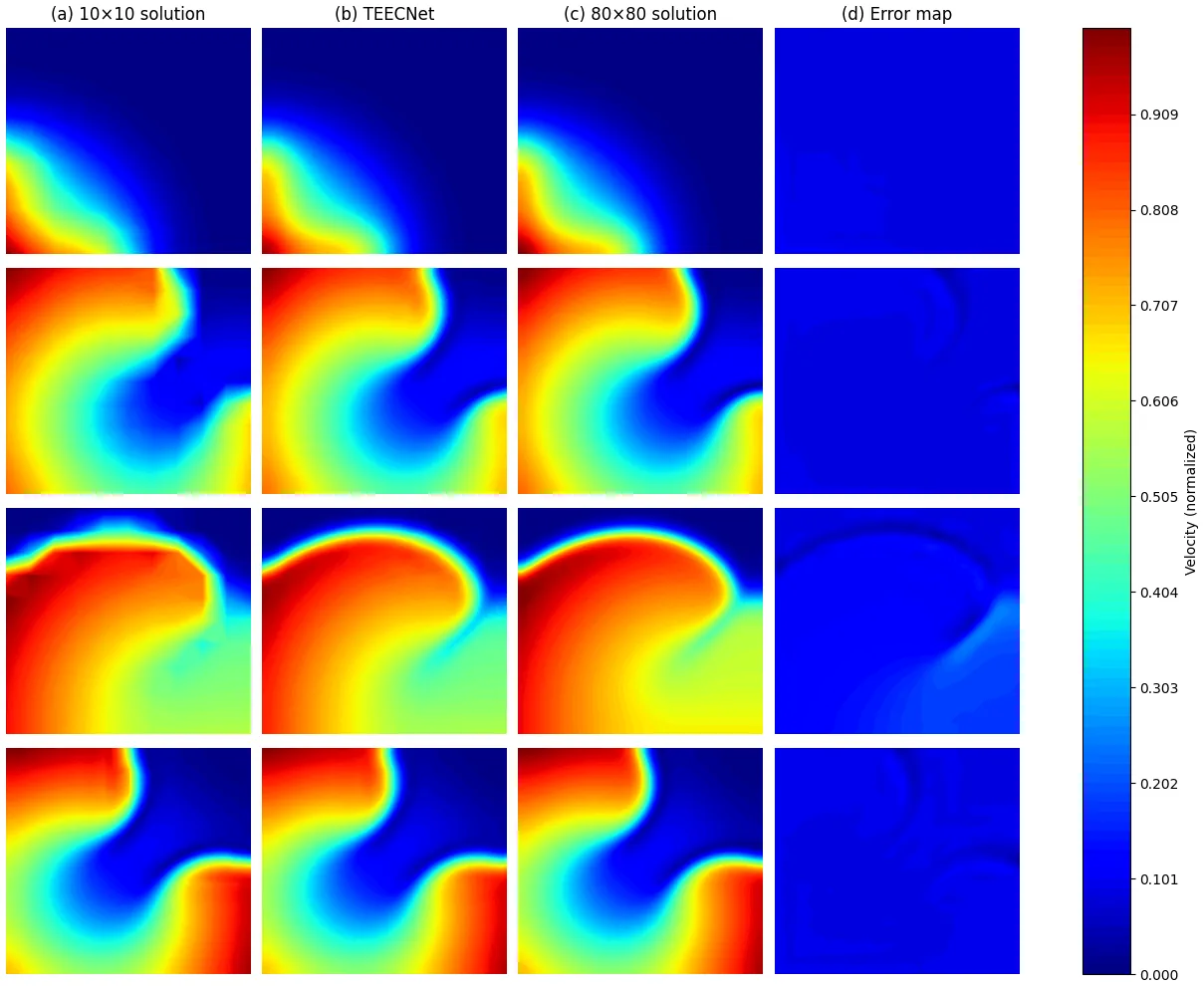
Grid of predicted fields across four samples comparing ground truth, TEECNet, a neural operator and GraphSAGE, with GraphSAGE showing white voids. — Four samples across the baselines. TEECNet and the neural operator both track the reference; GraphSAGE breaks.

Residual error maps across samples, with error concentrated in thin lines along the sharpest gradients. — What is left over sits in thin lines along the sharpest gradients — the field itself comes back clean.

The generalization result is the one I am proudest of. Five training resolution pairs, each evaluated on six test pairs: thirty combinations, one architecture, no retraining. Train on [20,40] or finer and every cell lands between R² 0.95 and 0.9995 — the best of them at 0.9995. Within a training pair the performance is flat across whatever test resolutions you hand it. The model simply does not care what resolution you evaluate it at.

On cost, the advantage widens as the machine shrinks: 1.75× faster than the neural operator on 48 cores (0.166 s vs 0.289 s), 3.2× faster on 12 (0.371 s vs 1.187 s). The tighter your compute budget, the more TEECNet wins by.

Then the cylinder wake, which is the hardest case here. From a coarse input that had smeared the wake into the free stream, TEECNet pulls the coherent shed structures and the low-velocity core back out.

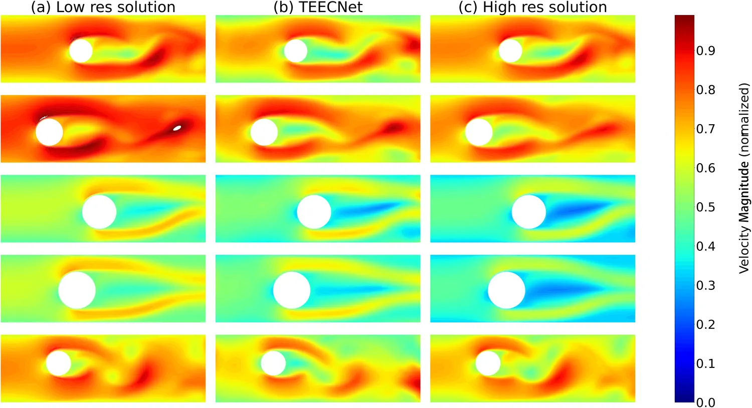
Five cylinder-wake cases in rows, each with three columns: low-resolution solution, TEECNet correction, and high-resolution solution. The TEECNet column closely matches the high-resolution column in every row. — Five MegaFlow2D cases. Column (a) is what the coarse solver produced, (c) is the fine-mesh truth, and (b) is TEECNet — read across each row and the correction lands on the reference.

MegaFlow2D

Alongside the method I released MegaFlow2D, the parametric flow dataset those cases come from. At the time every super-resolution paper reported on its own bespoke flow, so no two numbers were comparable. Both the method and the dataset are public, and the error-correction formulation became the base for the duct-design, domain-decomposition and vascular hemodynamics work that followed.

TEECNet code · MegaFlow2D dataset · Paper — J. Comput. Phys. 521 (2025) · MegaFlow2D — CPS-IoT Week 2023

← All projects · Research overview