Super-resolution for engineering duct design

Carnegie Mellon University · with Eaton Research Labs and the U.S. Army ERDC · 2023 – 2026 · Journal of Computing and Information Science in Engineering 26 (2026)

Six velocity-magnitude renders of a mixing elbow, arranged as two rows for 0-degree and 40-degree branch angles, showing coarse input, model prediction and high-resolution reference in near-identical detail.

An engineer changing a duct geometry wants an answer before the meeting ends. High-fidelity CFD gives them one the next morning. So the simulation stops being a design tool and becomes a sign-off step — you stop exploring and start confirming.

This is the work that closes that gap, and it is deployed in Eaton’s jet engine duct system design workflow.

5.5×faster than the high-fidelity simulation 100,000+parameterized CFD simulations generated <5%error in the flow quantities engineers size hardware against Deployedin Eaton's production design workflow

Run the cheap solver, then correct it

The pipeline keeps the numerical solver and adds a learned correction on top. A coarse mesh goes through the ordinary solver; a graph-based super-resolution model then maps that solution onto the fine mesh, using the geometry itself as the graph. Because the model reads an unstructured mesh directly, the same trained weights transfer across duct geometries instead of needing a new grid for each part.

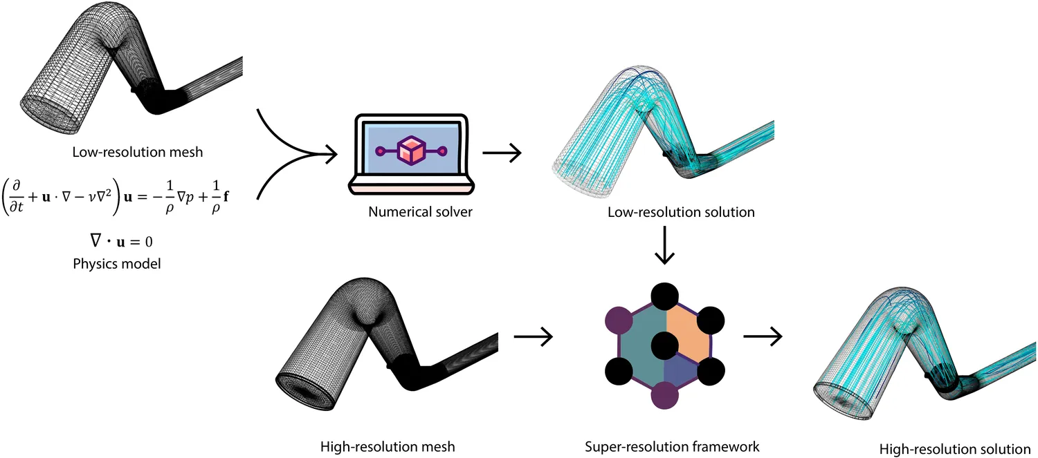
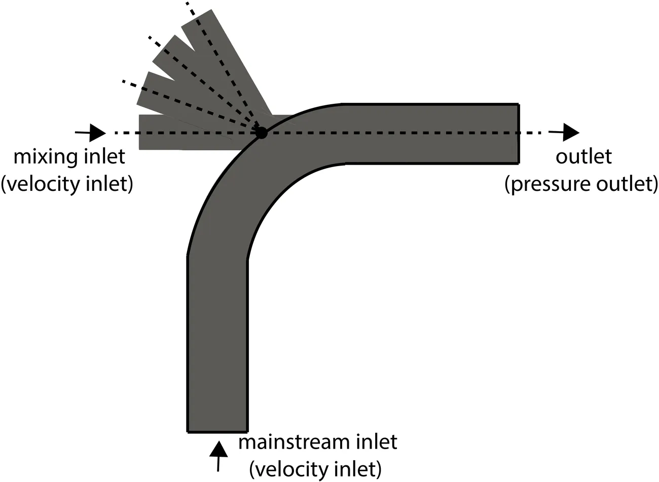
Pipeline diagram: a low-resolution mesh and the Navier-Stokes equations feed a numerical solver producing a low-resolution solution, which together with a high-resolution mesh feeds a graph-based super-resolution framework producing a high-resolution solution. — The solver stays. The learned correction takes its coarse output to the fine mesh, reading the geometry as a graph.

Training data came from a fully parameterized generator: more than 100,000 CFD simulations spanning geometries and boundary conditions, so the model sees the design space rather than a handful of examples from it.

Parameterized mixing-elbow geometry with the branch inlet angle marked as a varying design parameter. — The geometry is parameterized, so the training set covers the space an engineer will actually move through.

It holds across geometry

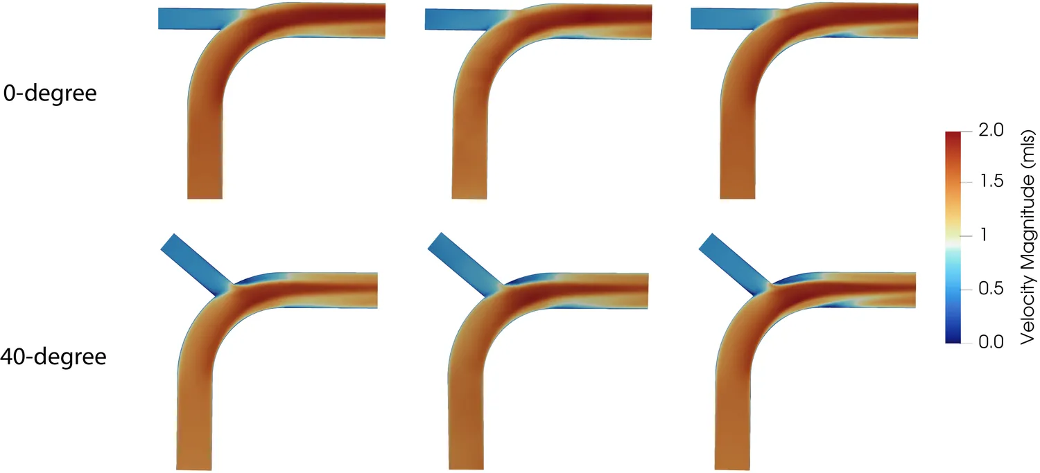
The header figure is the result that matters: two branch angles, and for each, coarse input against prediction against high-resolution reference. The prediction recovers the high-velocity core through the bend and the low-velocity wedge where the branch flow meets the main duct — the features that set pressure drop.

Velocity magnitude through a venturi section of the duct, comparing prediction against the high-resolution reference. — A venturi section: the model reproduces the acceleration through the throat and the recovery downstream.

What it costs

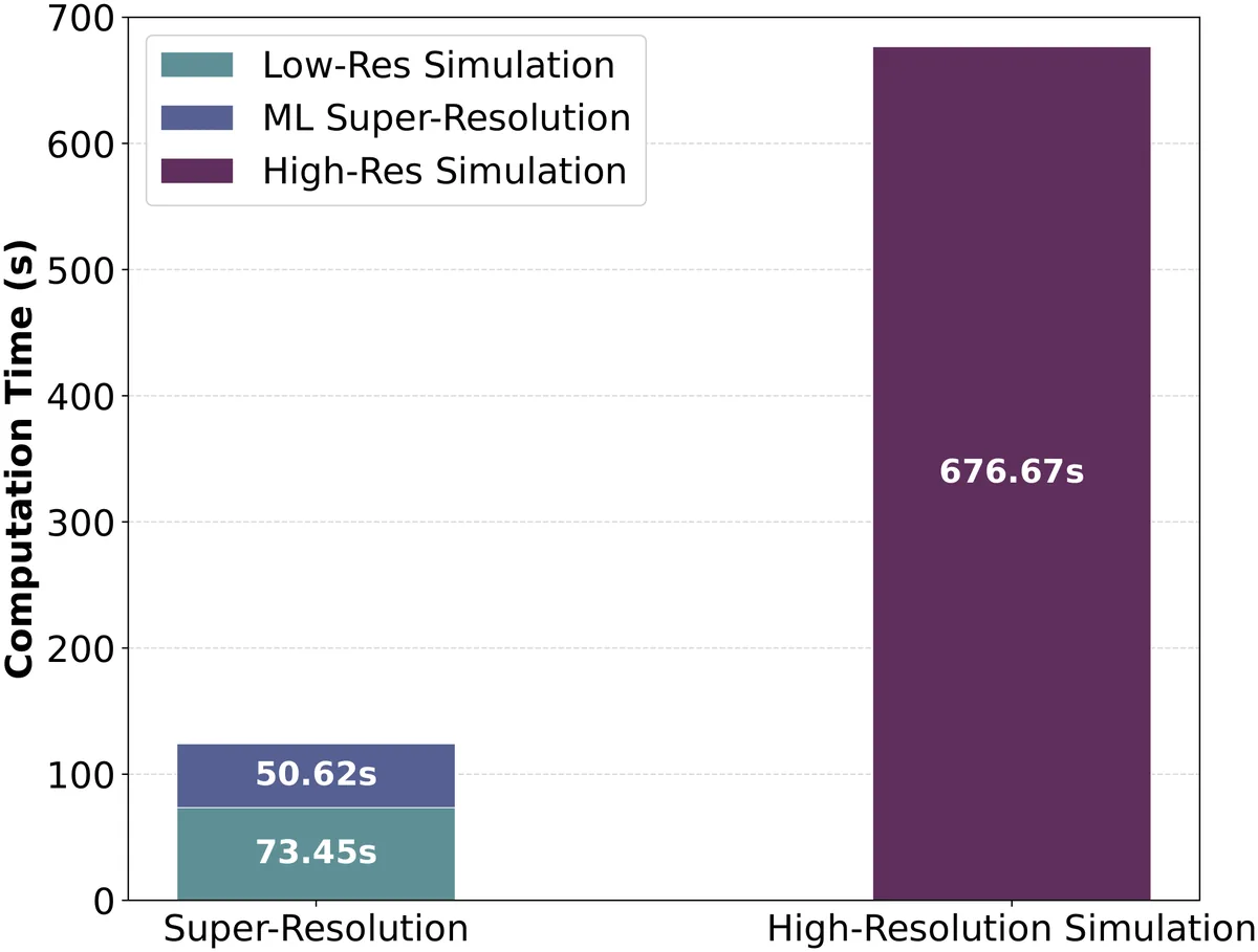
For the mixing elbow, high-fidelity CFD takes 676.67 s. The accelerated route takes 124.07 s — 73.45 s for the coarse simulation plus 50.62 s for the correction. That is a 5.5× speedup, and the coarse solver is the larger share of what remains.

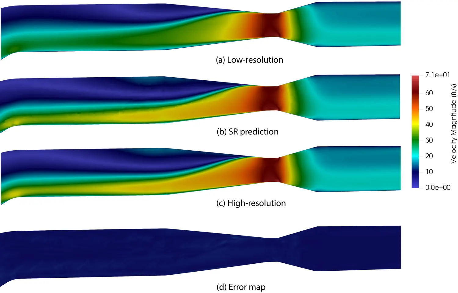
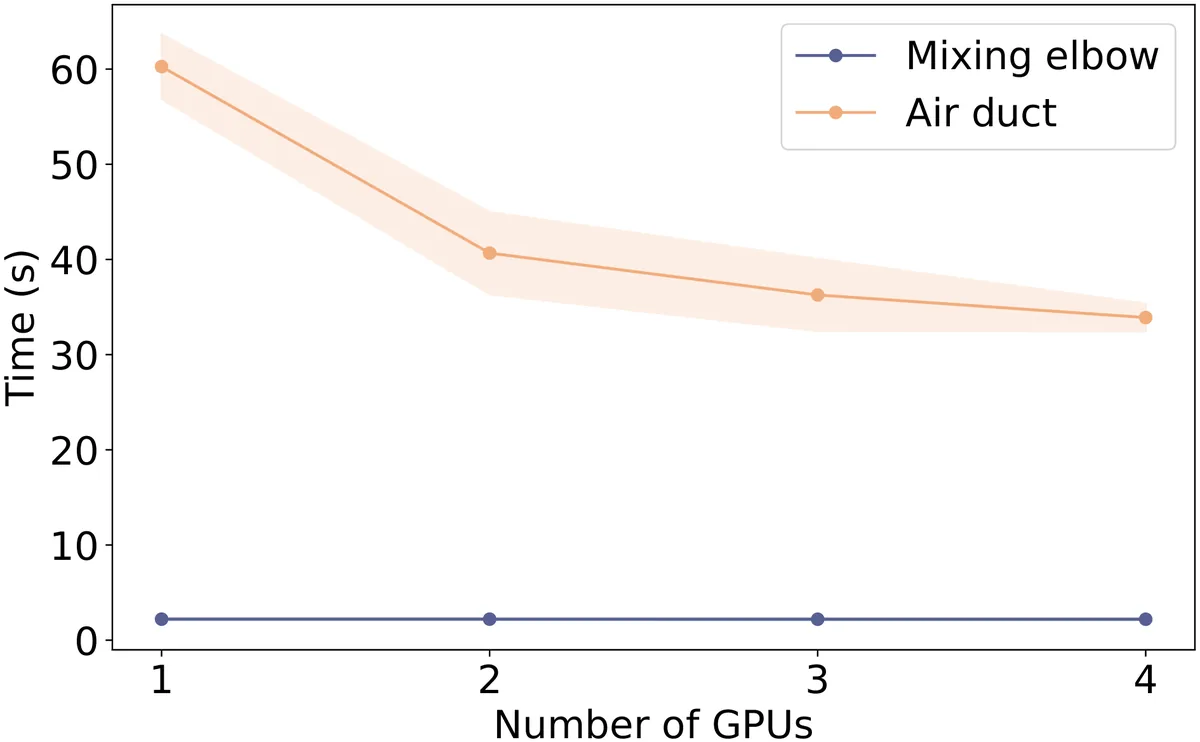
Stacked bar chart comparing 73.45 seconds of low-resolution simulation plus 50.62 seconds of ML super-resolution against 676.67 seconds for the high-resolution simulation. — 676.67 s of high-fidelity CFD against 124.07 s end to end.

The correction also distributes. On the larger air-duct case, inference drops from 60.3 s on one GPU to 33.9 s on four; the mixing elbow is small enough to finish in about 2 s regardless, which is the point at which the model has stopped being the constraint.

Inference time against number of GPUs for two cases: the air duct falling from about 60 seconds on one GPU to about 34 seconds on four, and the mixing elbow flat near 2 seconds. — Multi-GPU inference on the air duct. The elbow is already fast enough that adding GPUs changes nothing.

Paper — JCISE 26 (2026) · Conference version — IDETC-CIE 2025

← All projects · Research overview