Super-resolution for cardiovascular blood flow
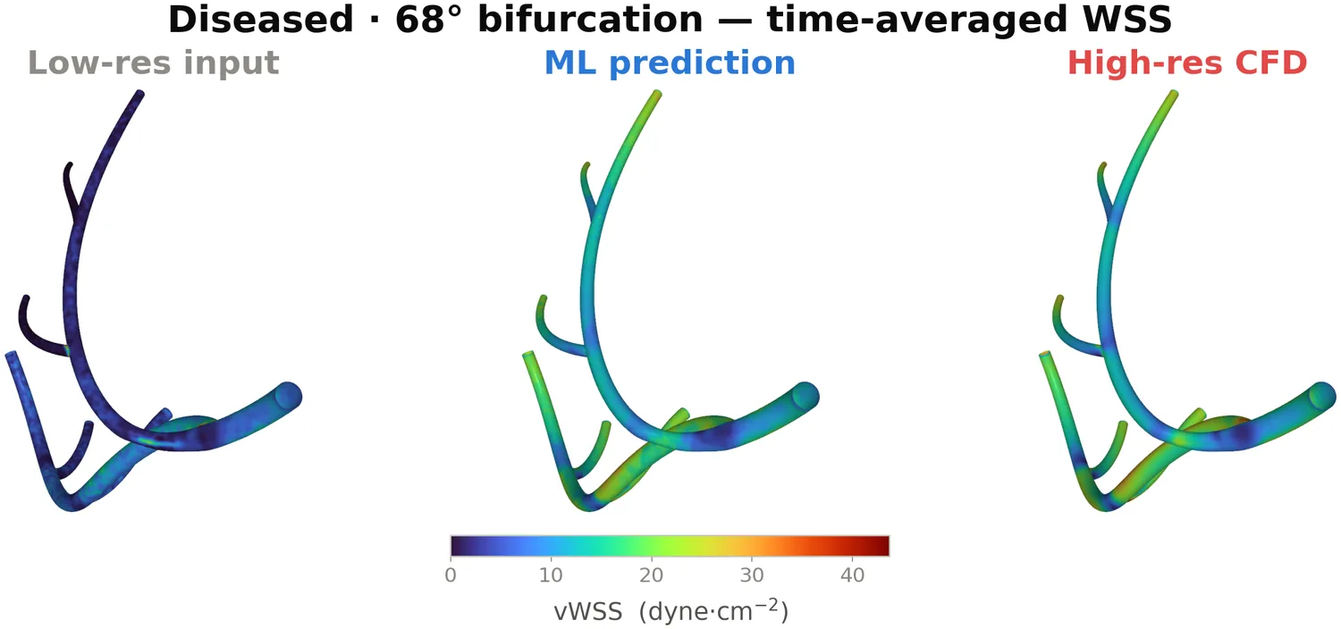
Wall shear stress is the number a cardiologist wants out of a coronary flow simulation. It is the force blood drags along the artery wall, and where it goes abnormal is where plaque is likely to be dangerous. It is also the single quantity a coarse mesh is worst at, because it is a gradient measured right at the wall — exactly where a cheap mesh has the fewest points.
So you are stuck. The simulation that gives you a trustworthy answer takes twelve hours per patient. The one that finishes over lunch tells you the wall is nearly quiescent when it is not. Look at the left panel above: that is the same artery, same blood, same heartbeat as the right panel. The coarse run just cannot see the shear.
Decompose, then correct
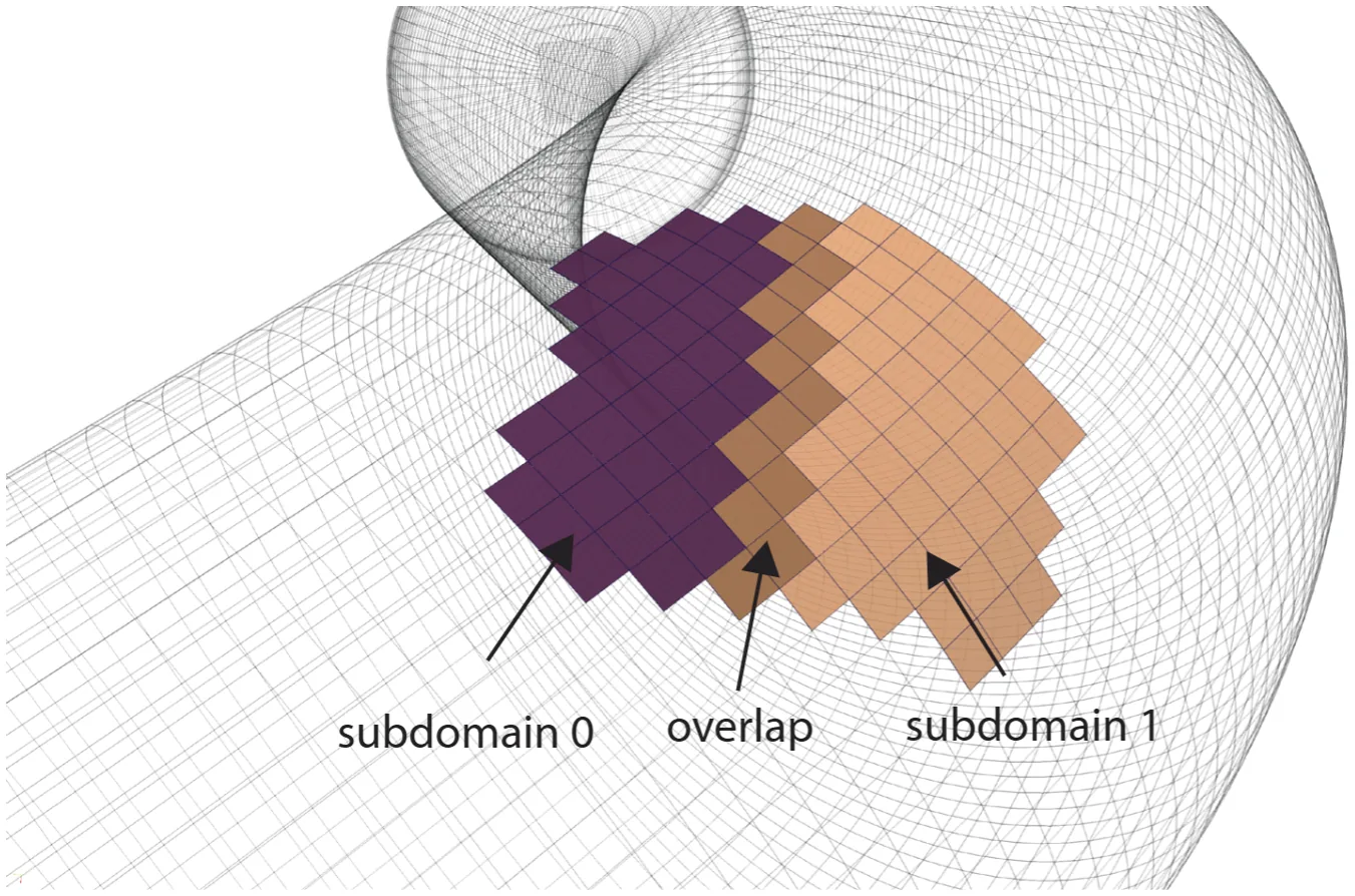
A neural network that has to look at a three-million-element artery all at once is a network that will run out of memory before it runs out of patience. The fix is to stop asking it to. The mesh is cut into overlapping subdomains, each small enough to reason about locally, and each is corrected independently. The overlap is the load-bearing part: it is what keeps the reconstruction continuous when the pieces are stitched back together, so you do not get seams where two subdomains disagree.
Training used 18 of the 24 synthetic left-coronary geometries — 12 healthy and 6 diseased, giving 193,536 subdomain samples — with 6 diseased geometries held out for testing. The geometries come from a parametric model of the left coronary tree, varying stenosis severity and lesion length.
Does it hold up over a heartbeat?
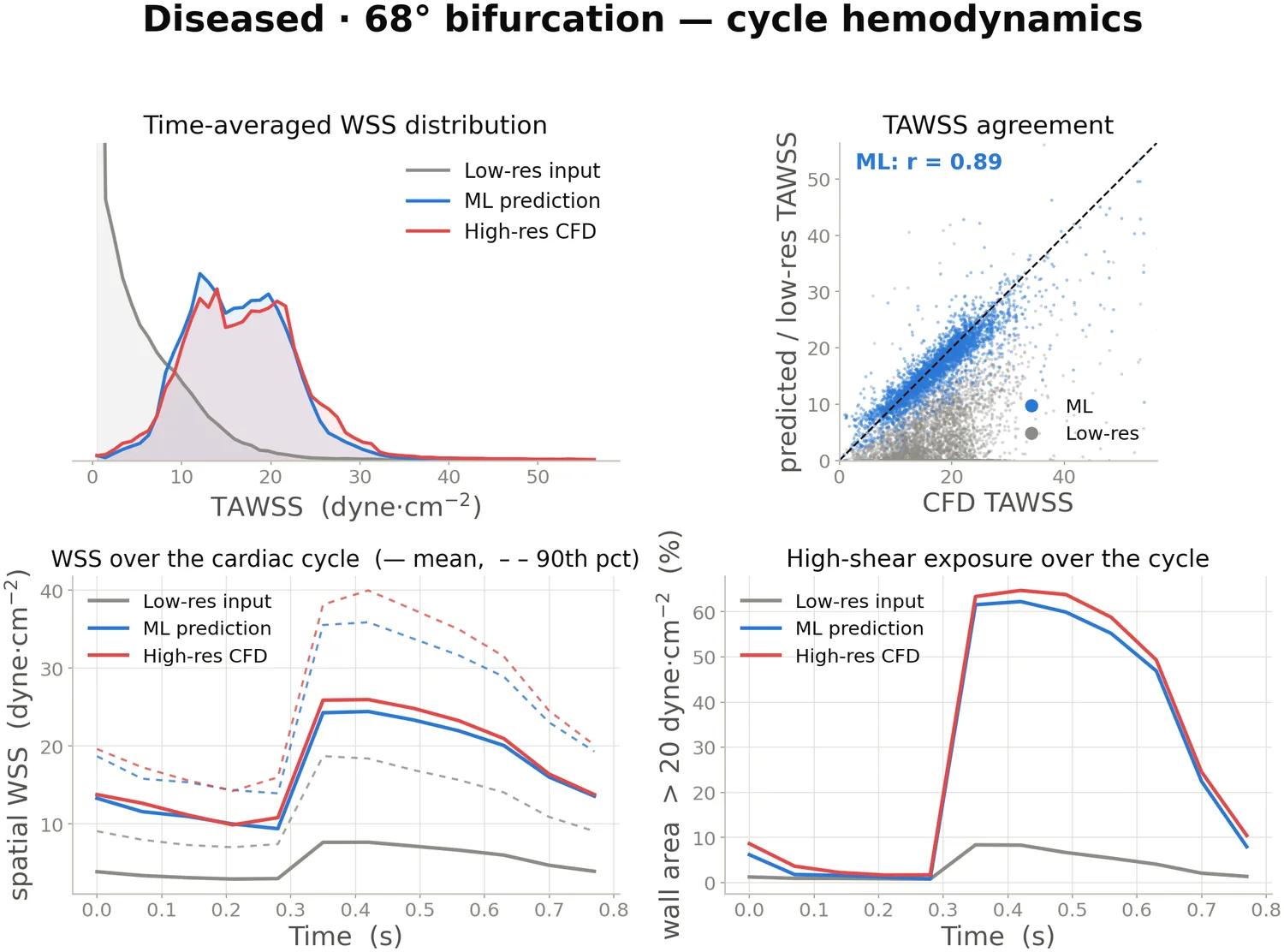
A time-averaged picture can hide a lot. Blood flow is pulsatile, and the clinically interesting moment is peak systole, when shear is highest and the model has the most to get wrong.
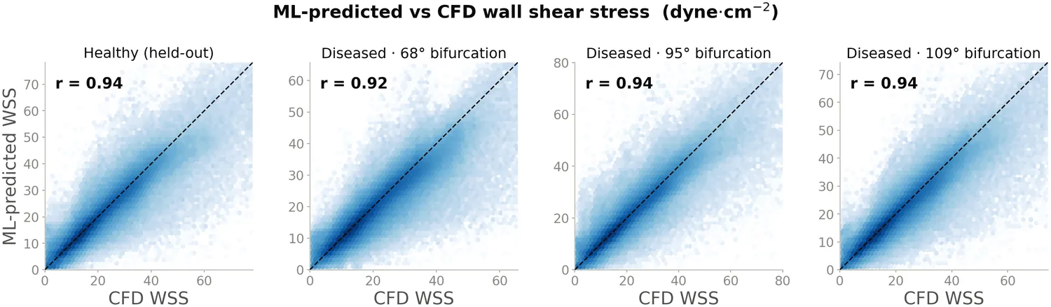
Across all four featured geometries, per-node predicted shear tracks the solver at r = 0.92–0.94 — including on the healthy geometry the model was never trained on.
The measure that actually decides something is high-shear exposure — how much of the wall crosses a clinical threshold, and when. At peak systole the model and the solver agree that roughly 62% and 65% of the wall exceeds 20 dyne·cm⁻². The coarse simulation puts it under 10%, which is not a small error but the opposite finding.
Generalizing across anatomy
One set of weights, four coronary trees, bifurcation angles from 68° to 122°. The high-shear bands land where each vessel’s own anatomy puts them — on the lesion neck, on the flow dividers — rather than in the same place every time. The model learned the hemodynamics, not a shape.
What it costs
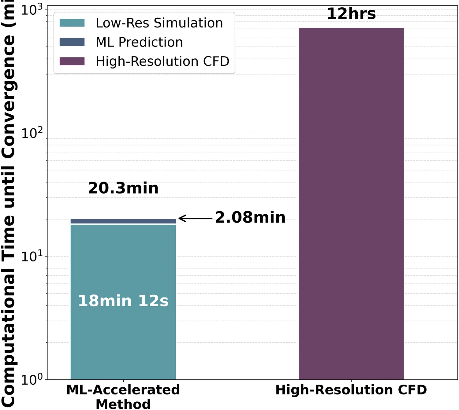
Twelve hours of high-fidelity CFD against 20.3 minutes end to end. The interesting detail is the split: 18 minutes 12 seconds of that is the coarse simulation you still have to run, and only 2.08 minutes is the network. The model is no longer the bottleneck — the cheap solver is.
Talk — APS-DFD 2025, Houston · Related paper — J. Comput. Phys. 538 (2025)