Adaptive local domain decomposition

Carnegie Mellon University · with Eaton Research Labs, ERDC and NSF ACCESS · 2024 · presented at APS-DFD 2024, Salt Lake City

A real flow is not one kind of physics. Near the wall it is laminar and orderly; a little further along it trips and breaks down; out in the free stream it is isotropic turbulence. A single network trained across all of that has to be a generalist, and generalists are mediocre everywhere — the loss averages over regimes that want different things from the model, and the compromise satisfies none of them.

The other half of the problem is size. The cost of a learned surrogate scales with the domain the way the solver’s does, so the model that worked beautifully on a benchmark box falls over on an engineering part.

0.66 → 0.80+R² after 20 rollout steps, undecomposed vs. decomposed 3physics regimes routed to their own sub-model

Locality is the licence to cut

The reason you are allowed to chop a domain up at all is that physical systems are local: two points close together are coupled far more strongly than two points far apart. An upwind scheme encodes this in its CFL condition; a spectral method encodes it in sparsity. If locality holds, then a subdomain plus a modest halo contains nearly everything needed to predict its interior — and the pieces can be distributed across GPUs without the physics noticing.

Testing that premise was its own piece of work. Enforcing bounded dependency areas in neural-operator propagation improves both error and learning dynamics — locality is not a compromise you accept for scale, it is a better way to build the model.

From the locality study I co-authored (Chen, Xu et al., J. Comput. Phys. 538, 2025): bounding how far information travels through the network improves accuracy rather than costing it.

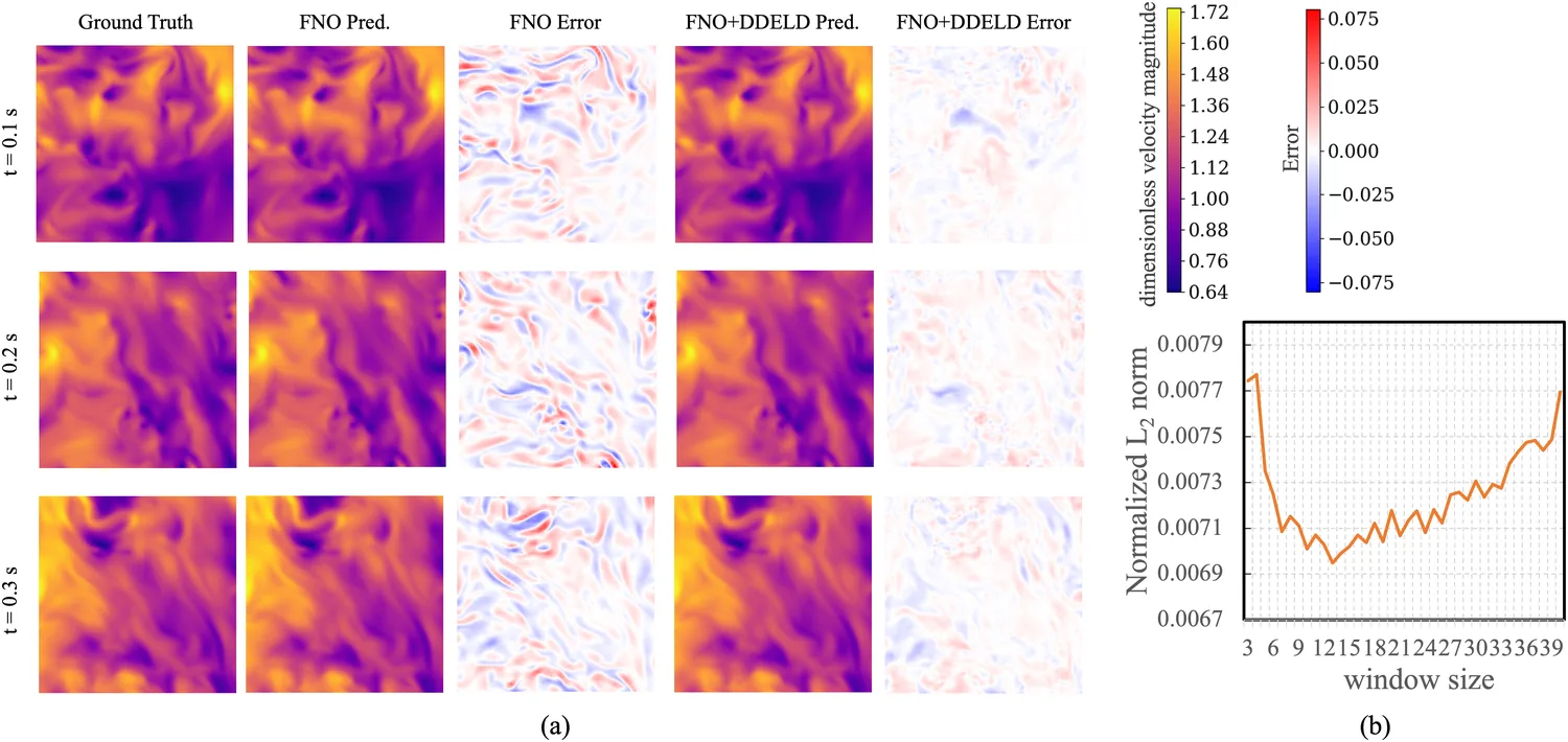
Describe the physics, then route it

If the domain is going to be cut anyway, the pieces need not all go to the same model. The question is how to tell which piece is which — and the answer has to come from the field itself, not from where the piece happens to sit.

One simulation, three sample locations: orderly near the inlet, breaking down in the middle, fully turbulent downstream.

The same three subdomains pulled out on their own. To a network these are three different problems wearing the same units.

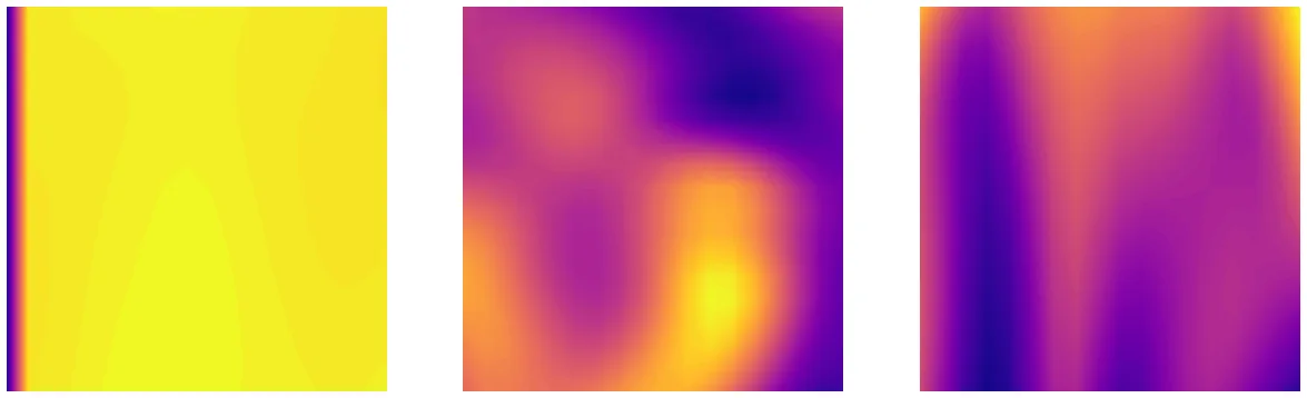
Each subdomain gets a descriptor and the descriptors get clustered, so the assignment is unsupervised — nobody labels a patch “turbulent”. Two descriptions were tried: the subdomain’s energy spectrum, and a PCA encoding of the field. Each was clustered under both a Euclidean and a Wasserstein metric.

Energy spectra at the three locations. The slopes differ enough to separate regimes without anyone labelling anything.

PCA with a Wasserstein metric characterized the physics best — Wasserstein compares whole distributions rather than points, which is the right instrument when what distinguishes two subdomains is the shape of their energy content.

The four descriptor–metric combinations, compared over a rollout. How you describe a subdomain changes what the routed models learn.

What it bought

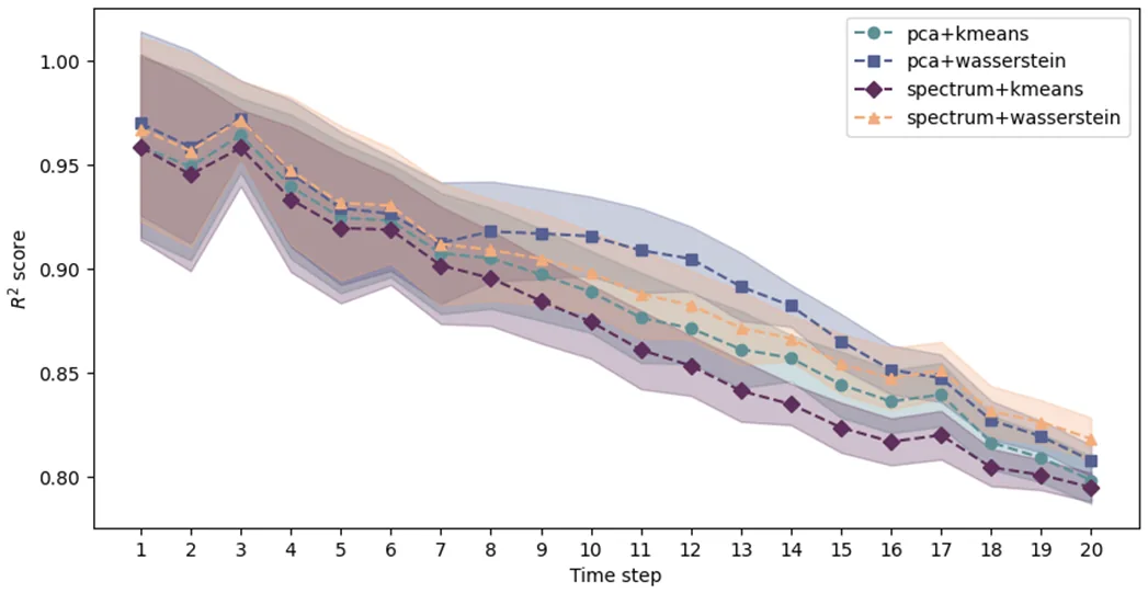
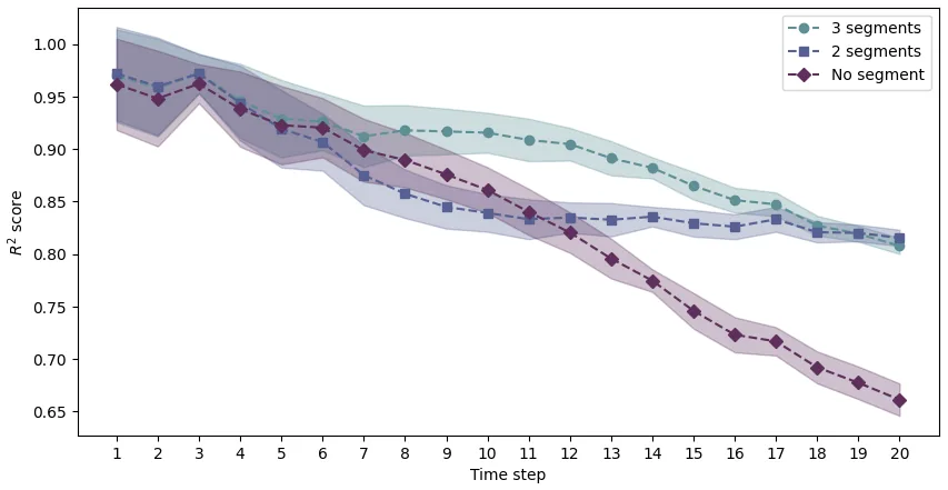
The test that matters for a surrogate is recurrent prediction: feed the model its own output and see how long it stays honest. Over twenty steps an undecomposed model decays to R² ≈ 0.66. The decomposed models hold above 0.80 — and the gap widens the further out you predict, which is exactly the direction you want it to run.

Twenty steps of recurrent prediction. The undecomposed model falls away; the decomposed ones do not.

Look back at the hero figure with that in mind. The prediction panel is a transitional boundary layer mid-breakdown — the hardest thing on this page for a single model to cover — and the error panel below it stays close to zero right through the transition.

Paper — J. Comput. Phys. 538 (2025) · Talk — APS-DFD 2024

← All projects · Research overview